
Numerical Solutions
STOMP uses Newton-Raphson linearization to solve the set of nonlinear algebraic equations formed by the discretized governing equations. This scheme has two major computational components: (1) to compute the Jacobian matrix and solution vector elements and (2) to solve the resulting linear system of equations.
Newton-Raphson Iteration
The nonlinearities in the coupled flow and energy transport system of equations are resolved through the application of the iterative Newton-Raphson technique. The Newton-Raphson linearization technique is an iterative method for solving nonlinear algebraic equations of the form

where f(x) is differentiable in x. The linearization concept approximates f(x) with suitable tangents.
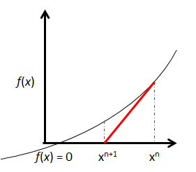
NR Iteration (Conceptual Plot)
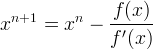
Each iteration yields a new estimate of x as the intersection of the tangent to the function f(x) at the previous estimate of x and the abscissa axis, according to
In this formulation f(x) is considered the equation residual. For convergent systems, the residual decreases quadratically with iteration. In multiple variable systems, as with the coupled flow and energy transport system, the scalar function, f(x), is replaced with a vector function R(x), according to
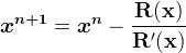
The vector function, R(x), represents the system of nonlinear algebraic equations produced from discretizing the conservation equations for component mass and energy. The vector of unknowns, x, represents the set of primary variables for the system, which are determined by the operational mode and phase conditions. This can be rewritten in terms of increments to the primary variables, according to
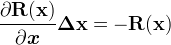
The partial derivatives shown above form the Jacobian matrix.
For simplification, a one-dimensional system involving the solution of the water mass, air mass, and energy conservation equations will be considered. The system of linear equations that result from applying the Newton-Raphson linearization technique to this system of nonlinear algebraic equations for a computational domain with “n” nodes is shown below.
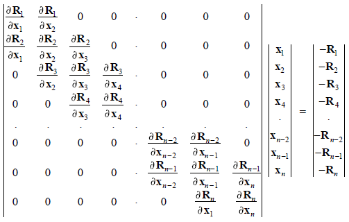
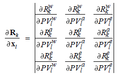
Here, each Jacobian matrix element represents a block matrix of order three, according to
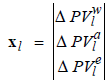
Each unknown vector element represents a vector of increments to the primary variables of order three, according to
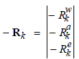
Each solution vector element represents a vector of equation residuals of order three, according to
![]() For a two-dimensional system involving the solution of the water mass, air mass, and energy conservation equations, the Jacobian matrix would contain two extra bands of block matrices: one below and one above the diagonal band. These extra bands would be located one half-band width from the main diagonal band, where the half-band width equaled the lesser of the number of nodes per row or column for a two-dimensional grid.
For a two-dimensional system involving the solution of the water mass, air mass, and energy conservation equations, the Jacobian matrix would contain two extra bands of block matrices: one below and one above the diagonal band. These extra bands would be located one half-band width from the main diagonal band, where the half-band width equaled the lesser of the number of nodes per row or column for a two-dimensional grid.
![]() A three-dimensional grid would contain four extra bands of block matrices, two below and two above the diagonal band. The furthest bands would be located one half-band width from the main diagonal band, where the halfband width equaled the least number of nodes in a plane. For example, a three-dimensional Cartesian grid with 20 nodes in the “X” coordinate direction, 30 nodes in the “Y” coordinate direction, and 40 nodes in the “Z” coordinate direction, would have a half-band width of 600.
A three-dimensional grid would contain four extra bands of block matrices, two below and two above the diagonal band. The furthest bands would be located one half-band width from the main diagonal band, where the halfband width equaled the least number of nodes in a plane. For example, a three-dimensional Cartesian grid with 20 nodes in the “X” coordinate direction, 30 nodes in the “Y” coordinate direction, and 40 nodes in the “Z” coordinate direction, would have a half-band width of 600.
Linear System Solvers
The linear system of equations produced during Newton-Raphson iteration is solved with either a direct or iterative linear system solver. The user must choose one of three solver options when requesting the source code.
(1) A banded matrix solution algorithm from LINPACK (solver=bd) is included with the source code as a direct solver.
The banded matrix solution algorithm was extracted from the LINPACK subroutines (Dongarra et al. 1979) for general nonsymmetric band matrices. The algorithm operates on band matrices by decomposing the matrix into an upper triangular and lower triangular matrix. The matrix product of the lower triangular matrix with the upper triangular matrix equals the original band matrix (i.e., A = L U, where A is the band matrix, L is the lower triangular matrix and U is the upper triangular matrix). The system of linear equations, A x = b, is solved with the above decomposition or factorization by solving successively L (U x) = b. This factorization procedure produces nonzero elements outside the bands of the original band matrix. If ml equals the half-band width of the Jacobian coefficient matrix (the Arid-ID engineering simulator produces band matrices with equal lower and upper band widths), then the two triangular factors have band widths of ml and 2ml. Storage must be provided for the extra ml diagonals. This is illustrated for a one-dimensional problem of five nodes and two-solved mass conservation equations. The Jacobian coefficient matrix for this problem would appear as shown.
Jacobian Coefficient Matrix
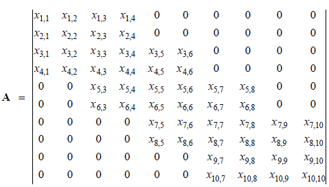
The band storage requires 3 ml + 1 = 10 rows of storage arranged as shown.
Storage Matrix
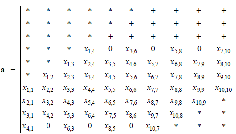
The * indicates elements which are never referenced but storage space must be provided. The + indicates elements which may be occupied during the factorization process. The original Jacobian coefficient matrix is referred to as A and its storage counterpart as a; then the columns of A are stored in the columns of a, and the diagonals of A are stored in the rows of a, such that the principal diagonal is stored in row 2 ml + 1 of a.
(2) A package of sparse iterative solvers, SPLIB (solver=sp), is included with the source code.
SPLIB offers several iterative methods for solving large sparse linear systems (Bramley and Wang 1995). STOMP implements all 13 iterative solvers and 7 preconditioning methods available from SPLIB.
The iterative methods included are:
- Bi-Conjugate Gradient (BICG)
- Conjugate Gradient for system A AT y = b, x = AT y (CGNE)
- Conjugate Gradient for system AT A x = AT b (CGNR)
- Conjugate Gradient Squared (CGS)
- Conjugate Gradients Stabilized (CGSTAB)
- Restarted generalized minimum residual (GMRES)
- Transpose-free QMR (QRMTF)
- Templates version of Conjugate Gradient Stablized (BICGS)
- Templates version of GMRES (GMREST)
- Jacobi Iteration (JACOBI)
- Gauss-Siedel (GAUSS)
- Successive Over-relaxation (SOR)
- Orthomin(m) (ORTHM)
The preconditioning methods included are:
- No preconditioner
- Incomplete LU factorization with s levels of fill (ILU(s))
- Modified incomplete LU factorizationwith s levels of fill and relaxation parameter ω (MILU(s,ω))
- Incomplete LU factorization with threshold dropping (ILUT(s,ω))
- Symmetric successive overrelaxation (SSOR(ω))
- Block diagonal with tridiagonal blocks (TRID(s)), where s is the block size
- Incomplete LU factorization without modification of off-diagonal elements (ILU0), the space saver version of ILU(0)
- Extended compressed incomplete modified Gram-Schmidt (ECIMGS(ω))
The user is referred to Bramley and Wang (1995) for more detailed information and references to each method
![]() The default iterative solver is CGSTAB and the default precondition option is ILU. These options are recommended for most problems, but the user may view or change these options in the psplib.F source file.
The default iterative solver is CGSTAB and the default precondition option is ILU. These options are recommended for most problems, but the user may view or change these options in the psplib.F source file.
(3) A conjugate gradient solver with multi-threading capabilities from PETSc (solver=petsc) is compatible with STOMP following the additional download.
The Portable, Extensible Toolkit for Scientific Computation (PETSc) is a suite of data structures and routines that provide the building blocks for the implementation of large-scale application codes on parallel (and serial) computers. Like SPLIB, PETSc offers several options for sparse linear system solvers. The user is referred to the PETSc manual or website for further information on each solver.
PETSc uses the MPI standard for all message-passing communication and is compatible in a multi-threaded mode for some STOMP operational modes, enabling parallel execution on a single workstation.
![]() The default iterative solver is bi-conjugate gradient stabilized (BiCGSTAB/KSPBCGS) and the default precondition option is incomplete LU factorization (ILU/PCILU). These options are recommended for most problems, but the user may view or change these options in the petsc.F source file.
The default iterative solver is bi-conjugate gradient stabilized (BiCGSTAB/KSPBCGS) and the default precondition option is incomplete LU factorization (ILU/PCILU). These options are recommended for most problems, but the user may view or change these options in the petsc.F source file.
![]() The banded matrix algorithm is appropriate for use with small to moderately sized problems (where the number of unknowns is on the order of less than 35,000).
The banded matrix algorithm is appropriate for use with small to moderately sized problems (where the number of unknowns is on the order of less than 35,000).
![]() Alternatively, the SPLIB and PETSc iterative solvers are more appropriate for larger problems (larger order numbers of unknowns).
Alternatively, the SPLIB and PETSc iterative solvers are more appropriate for larger problems (larger order numbers of unknowns).
![]() The PETSc solver tends to run a bit faster than the SPLIB solver. It also has multi-threading capabilities compatible with some STOMP modules.
The PETSc solver tends to run a bit faster than the SPLIB solver. It also has multi-threading capabilities compatible with some STOMP modules.
References
Bramley R and X Wang. 1995. SPLIB: A library of iterative methods for sparse linear system. Technical Report, Indiana Univeristy-Bloomington, Bloomington, IN-47405.
Dongarra, JJ., J Bunch, C Moler and GW Stewart. 1979. LINPACK User’s Guide. SIAM, Philadelphia, PA.