
Code Design (e)
The primary flow path for all operational modes of the eSTOMP simulator comprises three principal components: 1) initialization, 2) iteration, and 3) closure. During the initialization, global arrays are created that are used as shared memory. The information about the actual data distribution and locality can then be easily obtained whenever local data is important. A detailed flow diagram for these components is shown below:
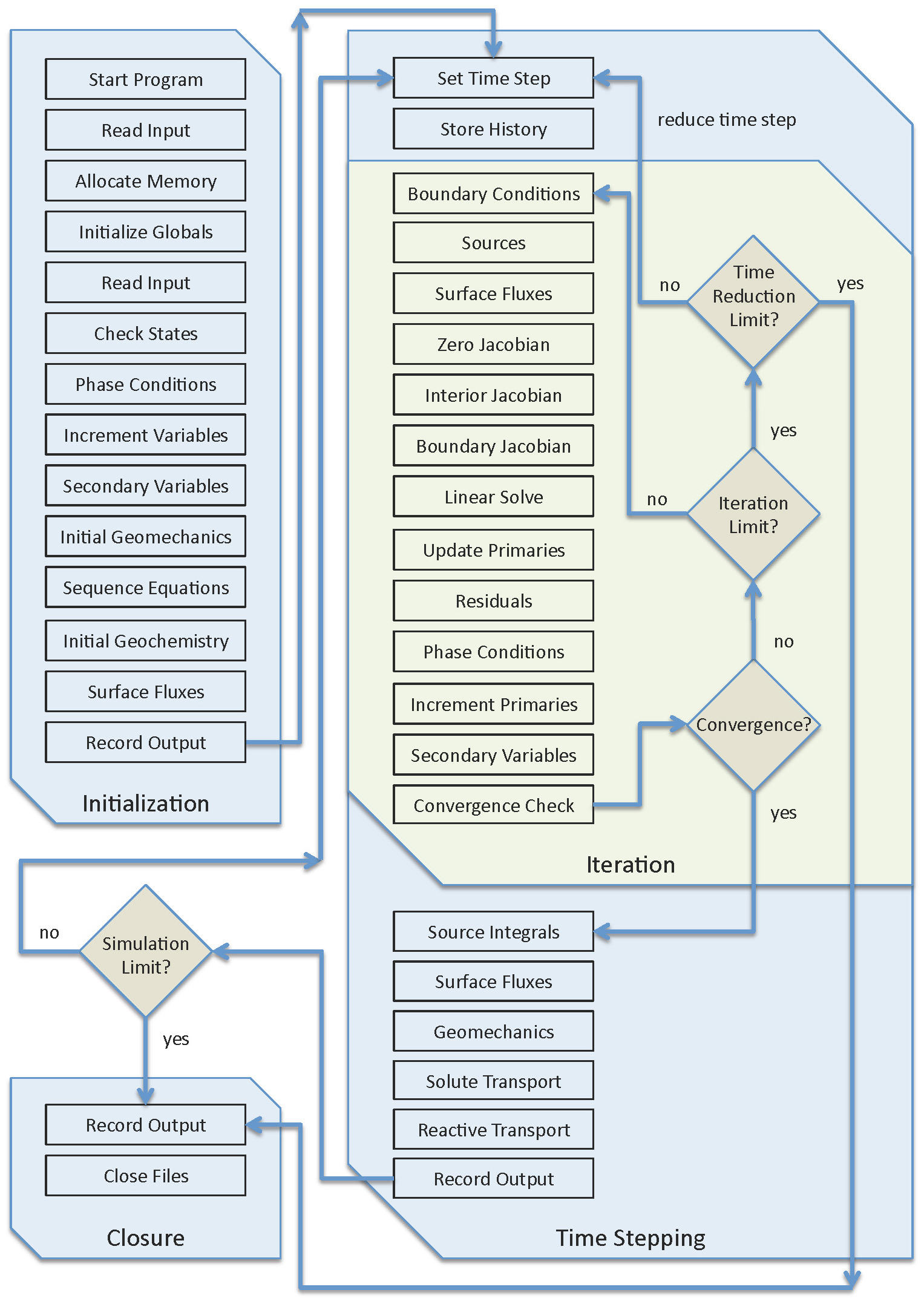
Figure 1. eSTOMP Flow Diagram
Initialization
The initialization component of the program is executed once per simulation. The routines in the initialization component are executed sequentially, as shown in Figure 1, from the program start to the start of the first time step.
During the initialization, a grid component as shown in the following diagram is first created to separate the implementation of the grid data structures and the parallel operations required to update grid “ghost” nodes (neighboring grid nodes that are owned by other processors) from the remainder of the application code. The grid component is used to distribute data across processors using domain decomposition, provide a mapping from local numbering scheme to global numbering scheme, manage the creation and destruction of data fields on the grid and set up the communication that allows the application to update ghost node, fields with data from other processors. The data model that the grid component supports describes the grid that is distributed across multiple processors in terms of nodes extended to incorporate ghost nodes, connections between nodes, and boundary connections on each processor.
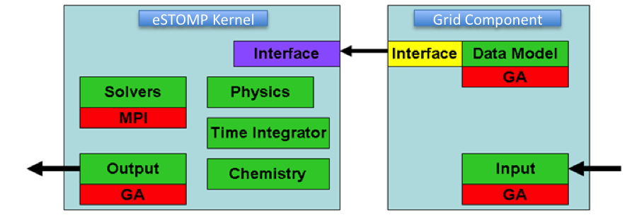
Figure 2. Schematic diagram of eSTOMP code showing the relationship of different functionalities and communication libraries. The boxes in green show different functionalities (except for the data model) that could be extracted as individual components in the future. The grid interface is implemented in the grid component and used in the eSTOMP kernel. The red boxes show the parallel communication libraries used to implement the different functionalities.
During initialization, the input file is read twice. The first read of the input file is used to allocate and initialize memory for all the global variables (i. e. , those variables passed among routines via modules). The second read of the input file is used to define the problem. The input file readers are not foolproof but do report error messages when input errors are noted. Once the input file has been successfully read twice, the initial states are checked for thermodynamic consistency, phase conditions are established, and the primary variables are selected for every grid cell. The next stage of initialization involves computing all the secondary variables at grid cells and boundary surfaces. If geomechanics calculations are included in the simulation, then the initial stress state of the domain is established. If coupled wells are included in the simulation, then the well trajectories are determined and the wells are equilibrated with the formation. Once the well trajectories are defined, the coupled conservation equations and coupled well equations are sequenced such that the band width of the Jacobian matrix is minimized. If geochemistry calculations are included in the simulation, then the initial chemical state of the system is established. With the initial primary and secondary variables computed, the next stage of initialization is to compute the initial surface fluxes at both internal surfaces and boundary surfaces (e. g. , volumetric phase flux, component advective/diffusive flux, heat flux). The final initialization stage is to record user requested output to the various output files (i. e. , output, plot. xxx, and surface). If a zero-time-step simulation is requested, the simulator stops at the end of the initialization, after recording output. This option is very useful for computing property values or examining initial states.
Iteration
The iteration component of the program contains a pair of nested loops. The outer loop performs time stepping and the inner loop performs Newton-Raphson iteration.
The time stepping component is where the simulator loops over time, with each time-step loop solving for the conditions at a new point in time. Geomechanics, reactive transport (geochemistry), and solute transport are solved sequentially with the coupled multifluid flow and heat transport. Each new time step begins with the assignment of a time step, which is determined from the previous time step parameters (e. g. , time step and convergence) and user input (e. g. , maximum time step, minimum time step, time-step acceleration factor, output times, boundary condition times, source times, coupled well times). The next step is to store the old time step values of the primary and secondary variables. Old-time-step values of fluxes are not stored. Next, boundary conditions and sources at the new time step are assigned. Fluxes across the interior and boundary surfaces are then computed. The Jacobian matrix, solution vector, and problem vector are all set to zero. The Jacobian matrix and problem vector are then loaded for all active nodes and interior surfaces (i. e. , non-boundary surfaces). The Jacobian matrix and problem vector is then corrected for boundary surface fluxes. At this point the Jacobian matrix and problem vector are complete and the linear system is either solved directly with a banded solver or iteratively. The resulting solution vector from the linear system solve contains corrections (updates) to the primary variables. The primary variables are then updated and residuals (errors) in the conservation equations are determined. The updated primary variables are then used to establish new phase conditions and a new primary variable set for each grid cell. Increments to the primary variables for the numerical derivatives are determined, and the secondary variables are computed using native and incremented primary variables. Convergence is then established using the conservation equation residuals; where the highest relative residual across the computational domain determines convergence.
- Termination of the Newton-Raphson loop occurs upon successful convergence or with an iteration limit violation.
- Termination of the time-stepping loop occurs due to the simulation limit or a time step reduction limit violation.
- It should be noted that "Solute Transport" is shown as a single routine on the STOMP flow diagram; however, it comprises several transport routines within a solute loop.

Figure 2. Transport Solution Flow Diagram
Closure
The closure routines are executed at the completion of a simulation (regardless of the termination cause).