
Boundary Conditions Description (G)
Overview
Boundary conditions are the mechanism by which the user can specific state conditions or fluxes across the surfaces of grid cells. Boundary conditions are always applied to grid-cell surfaces and in the case of state conditions are applied at the point of the centroid of the grid-cell surface. In STOMP boundary conditions can only be applied to three types of grid cell surfaces: 1) surfaces on the boundary of the computational domain, 2) surfaces between active and inactive grid cells, and 3) surfaces along the boundary of an internal split in the computational domain. Boundary conditions are always applied to active grid cells and the grid-cell surface to which the boundary condition is applied is in reference to the active grid cell. Grid cells in STOMP have hexahedral geometries and are defined by 8 vertices. Each of the 6 grid-cell surfaces are named according to their orientation in the computational coordinate system (CCS), as described in Table 1 and shown in Figure 1. Grid-cell surfaces are not oriented with respect to the global Cartesian coordinate system (GCS) that defines the location of the grid-cell vertices. The types of boundary conditions which can be applied to surfaces and the specification of those boundary conditions varies among the STOMP Operational Modes, but the application concepts are similar. Boundary conditions require that the user specify the location of the boundary surface and the time history of state condition or flux.

Figure 1. Grid-cell surface naming
Table 1. Grid-Cell Surface Naming and Surface Normals with respect to the computational coordinate system (CCS).
Grid-Cell Surface Name | GCS Number | GCS Orientation | GCS Position | GCS Surface Normal |
|---|---|---|---|---|
| Bottom | -3 | X-Y Trending | Lower Surface | Negative Z-Direction |
| South | -2 | X-Z Trending | Lower Surface | Negative Y-Direction |
| West | -1 | Y-Z Trending | Lower Surface | Negative X-Direction |
| East | 1 | Y-Z Trending | Upper Surface | Positive X-Direction |
| North | 2 | X-Z Trending | Upper Surface | Positive Y-Direction |
| Top | 3 | X-Y Trending | Upper Surface | Positive Z-Direction |
Application Notes
The Boundary Conditions Card is an optional card, but is generally necessary to simulate a particular problem. Boundary surfaces with undeclared boundary conditions are by default zero flux boundaries. The application of boundary conditions in the STOMP Simulator varies across operational modes. Most operational modes allow great flexibility in specifying boundary conditions; whereas, other operational modes limit this flexibility. For those operational modes with full flexibility and multiple phases, the user is not required to have phase equilibrium between phases crossing the boundary surface. For example, it is possible to specify aqueous injection and gas withdrawal concurrently on the same boundary surface for some operational modes. The cost of this flexibility is that the specification of boundary conditions becomes a responsibility of the user.
Application of boundary conditions requires an appropriate conceptualization of the physical problem and translation of that conceptualization into boundary condition form. The variety of boundary condition types available in the simulator should afford the user the flexibility to solve most subsurface flow and transport problems. The boundary condition card reader within the simulator performs limited error checking on the boundary condition inputs. An error free boundary condition card does not guarantee the user has not created an ill-posed problem or an execution that will successfully converge. For example, a mistake frequently made by users is to specify infiltration rates at the top of a column with positive fluxes. While this input would be perfectly acceptable to the boundary condition input reader, the specified condition would actually withdraw flux from the top of the column since the z-axis and z- direction flux are positive in the upward direction.
Time Varying Boundaries
Boundary conditions in STOMP can vary with time in three ways: 1) linear variation, 2) stepped variation, and 3) cyclic variation. Time varying boundary conditions are created by specifying boundary conditions at multiple points in time; where, time is in reference to the simulation time declared on the Solution Control Card. The first time point of a boundary condition is the start time for the boundary condition and the final time point of a sequence of boundary condition times is the stop time. Two concurrent boundary conditions on the same boundary surface are not permitted. The boundary condition parameters vary between time points in a linear fashion. To create stepped variation in boundary conditions multiple time points are specified with the same times. Cyclic variation of boundary conditions repeats the time sequence until the simulation completes. A boundary condition declared with a single boundary time implies that the boundary condition is time invariant, and the specified boundary time represents the start time for the boundary condition. Prior to the start time the boundary surface will be assumed to be of type zero flux. The specified boundary condition will remain in effect from the start time until the execution is completed. If a boundary condition is declared with multiple boundary times, then the first time listed equals the start time, the last time listed equals the stop time, and the intermediate times are transition points. For simulation times outside of the start and stop time limits, zero flux boundary conditions apply.
Boundary Condition Types
There are three general types of boundary conditions: 1) Dirichet, 2) Neumann, and 3) Robin, all named after mathematicians. The Dirichlet boundary condition, named after the French mathematician, Peter Gustav Lejeune Dirichlet, and also known as the first-type boundary condition, is one where a state variable (e.g., temperature, pressure, concentration) is specified on the boundary surface. The state variable is applied at the centroid of the boundary surface. The Neumann boundary condition, named after the German mathematician, Carl Gottfried Neumann, and also known as the second-type boundary condition, is one where the derivative of a variable is specified on the boundary. In the case of STOMP the specification is one of flux and not the derivative directly. For example, a pure Neumann boundary condition for energy would be that of the derivative of temperature with distance, but in STOMP the heat flux is specified. The Robin boundary condition, named after the French mathematician, Victor Gustave Robin, is a linear combination of the Dirichlet and Neumann boundary conditions. Robin type boundary conditions are not generally available in STOMP, except for those operational modes that consider interactions between the atmosphere and ground surface.
The discretized forms for Darcy mass flux and diffusive mass flux rates of water are modified for a Dirichlet aqueous phase boundary condition on a “west” boundary (WB) surface, according to
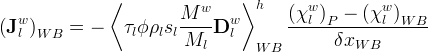
For the salt and solute mass conservation equations, a Dirichlet boundary condition on the “west” surface produces a modification to the discretized conservation equations, according to:

Symbols | |
|---|---|
 |
advective water mass flux in aqueous phase, kg/m2 s |
 |
diffusive-dispersive water flux for the aqueous phase, kg/m2 s |
 |
intrinsic permeability tensor, m2 |
 |
unit gravitational direction vector |
 |
diffusion-dispersion tensor of water for aqueous phase, m2/s |
 |
solute mass conservation equation coefficient for node ζ |
 |
acceleration of gravity, m/s2 |
 |
solute concentration, 1/m3 |
 |
aqueous relative permeability |
 |
molecular weight of water, kg/kmol |
 |
molecular weight of aqueous phase, kg/kmol |
 |
solute source rate, 1/s |
 |
salt mass source rate, kg/s |
 |
aqueous liquid pressure, Pa |
 |
solute decay rate constant, 1/s |
 |
actual aqueous liquid saturation |
 |
salt concentration, kg/m3 |
 |
volume of the aqueous phase, m3 |
 |
time step, s |
 |
node spacing across surface WB, m |
 |
dynamic viscosity of fluid in aqueous phase, kg/(m s) |
 |
density of fluid in aqueous phase, kg/m3 |
 |
aqueous phase tortuosity |
 |
diffusive porosity |
 |
mole fraction of water in aqueous phase |
 |
mass fraction of water in aqueous phase |
| subscript B |
bottom |
| subscript E |
east |
| subscript N |
north |
| subscript P | center or local node |
| subscript S |
south |
| subscript T |
top |
subscript WB |
west boundary surface |
 |
arithmetic interfacial averaging at surface WB |
 |
harmonic interfacial averaging at surface WB |
 |
upwind or donor cell interfacial averaging at surface WB |
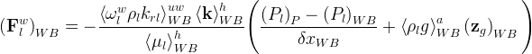
For example, the discretized form for Darcy mass flux of water is modified for a Neumann boundary condition on a “west” boundary (WB) surface, according to

Sufficient information is needed to fix the thermodynamic and hydrologic state on the boundary surface. Calculation of phase pressures from phase volumetric flow rates requires an iterative solution because averaged values of properties (e.g., relative permeability) are nonlinear functions of the phase pressure on the boundary. To avoid an iterative solution of the phase pressure on the boundary phase pressures are computed assuming a unit relative permeability, according to
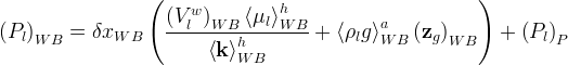
for a “west” boundary surface.
Symbols | |
|---|---|
 |
advective water mass flux in aqueous phase, kg/m2 s |
 |
acceleration of gravity, m/s2 |
 |
intrinsic permeability tensor, m2 |
 |
aqueous liquid pressure, Pa |
 |
Darcy velocity of water component in the aqueous phase, m/s |
 |
Darcy velocity of the aqueous phase, m/s |
 |
unit gravitational direction vector |
 |
node spacing across surface WB, m |
 |
dynamic viscosity of fluid in aqueous phase, kg/(m s) |
 |
density of fluid in aqueous phase, kg/m3 |
 |
mass fraction of water in aqueous phase |
| subscript P | center or local node |
| subscript WB | west boundary surface |
 |
arithmetic interfacial averaging at surface WB |
 |
harmonic interfacial averaging at surface WB |
 |
upwind or donor cell interfacial averaging at surface WB |